PubMatrixR with Ligand Receptors

Introduction

This vignette applies PubMatrixR to a real biology question: how do WNT ligands and their receptors show up together in the literature? WNT signaling touches cell fate, tissue patterning, and stem cell maintenance, and the ligand-receptor pairings are not one-to-one. Some ligands are studied constantly alongside certain receptors and barely mentioned with others.

The example below compares 19 WNT ligands against 15 receptors (FZD1-10, LRP5/6, ROR1/2, RYK), producing a 15x19 grid of PubMed co-occurrence counts.

library(PubMatrixR)
library(knitr)
library(kableExtra)
library(dplyr)
library(pheatmap)
library(ggplot2)

A <- c(
  "WNT1", "WNT2", "WNT2B", "WNT3", "WNT3A", "WNT4", "WNT5A", "WNT5B",
  "WNT6", "WNT7A", "WNT7B", "WNT8A", "WNT8B", "WNT9A", "WNT9B",
  "WNT10A", "WNT10B", "WNT11", "WNT16"
)

B <- c(
  "FZD1", "FZD2", "FZD3", "FZD4", "FZD5", "FZD6", "FZD7",
  "FZD8", "FZD9", "FZD10", "LRP5", "LRP6", "ROR1", "ROR2", "RYK"
)

Running the search

The live call below queries PubMed directly. A grid this size means 285 pairwise searches, so it can take a while. This vignette skips the live call and uses a synthetic matrix instead, so the page builds without depending on NCBI being reachable. Swap in your own gene lists and run the live version for real numbers.

NCBI API Key (Recommended)

For better performance and higher rate limits, we recommend obtaining an NCBI API key:

Without API key: 3 requests per second
With API key: 10 requests per second

To obtain your free NCBI API key, visit: https://support.nlm.nih.gov/kbArticle/?pn=KA-05317

Once you have your API key, pass it to PubMatrix() like this:

result <- PubMatrix(
  A = A,
  B = B,
  API.key = "your_api_key_here",
  Database = "pubmed"
)

For live rendering, this vignette picks up the key from the NCBI_API_KEY environment variable instead of hardcoding it, so no key is stored in the file:

NCBI_API_KEY=your_api_key_here PUBMATRIX_LIVE_VIGNETTE=true \
  Rscript -e 'pkgdown::build_site()'

current_year <- as.integer(format(Sys.Date(), "%Y"))
result <- PubMatrix(
  A = A,
  B = B,
  API.key = ncbi_api_key,
  Database = "pubmed",
  daterange = c(1990, current_year),
  outfile = "pubmatrix_result"
)

# Offline deterministic example used for vignette rendering/package checks.
result <- outer(seq_along(B), seq_along(A), function(i, j) {
  10 + (i * 5) + (j * 4) + ((i + j) %% 5) * 2 + ((i * j) %% 6)
})
result <- as.data.frame(result, check.names = FALSE)
colnames(result) <- A
rownames(result) <- B

Which genes get the most attention

Before the pairwise grid, it’s worth checking which individual genes are studied the most. The bar charts sum each gene’s row or column and color it by its strongest partner on the other list, which shows which receptor tends to dominate the literature for a given ligand, and the reverse.

# Create data frame for List A genes (rows) colored by List B genes (columns)
a_genes_data <- data.frame(
  gene = rownames(result),
  total_pubs = rowSums(result),
  stringsAsFactors = FALSE
)

# Add color coding based on max overlap with B genes
a_genes_data$max_b_gene <- apply(result, 1, function(x) colnames(result)[which.max(x)])
a_genes_data$max_overlap <- apply(result, 1, max)

# Create data frame for List B genes (columns) colored by List A genes (rows)
b_genes_data <- data.frame(
  gene = colnames(result),
  total_pubs = colSums(result),
  stringsAsFactors = FALSE
)

# Add color coding based on max overlap with A genes
b_genes_data$max_a_gene <- apply(result, 2, function(x) rownames(result)[which.max(x)])
b_genes_data$max_overlap <- apply(result, 2, max)

# Plot A genes colored by their strongest B gene partner
p1 <- ggplot(a_genes_data, aes(x = reorder(gene, total_pubs), y = total_pubs, fill = max_b_gene)) +
  geom_bar(stat = "identity") +
  coord_flip() +
  labs(
    title = "List A Genes by Publication Count",
    subtitle = "Colored by strongest List B gene partner",
    x = "Genes (List A)",
    y = "Total Publications",
    fill = "Strongest B Partner"
  ) +
  theme_minimal() +
  theme(legend.position = "bottom") +
  scale_fill_viridis_d()


# Plot B genes colored by their strongest A gene partner
p2 <- ggplot(b_genes_data, aes(x = reorder(gene, total_pubs), y = total_pubs, fill = max_a_gene)) +
  geom_bar(stat = "identity") +
  coord_flip() +
  labs(
    title = "List B Genes by Publication Count",
    subtitle = "Colored by strongest List A gene partner",
    x = "Genes (List B)",
    y = "Total Publications",
    fill = "Strongest A Partner"
  ) +
  theme_minimal() +
  theme(legend.position = "bottom") +
  scale_fill_viridis_d()


print(p1)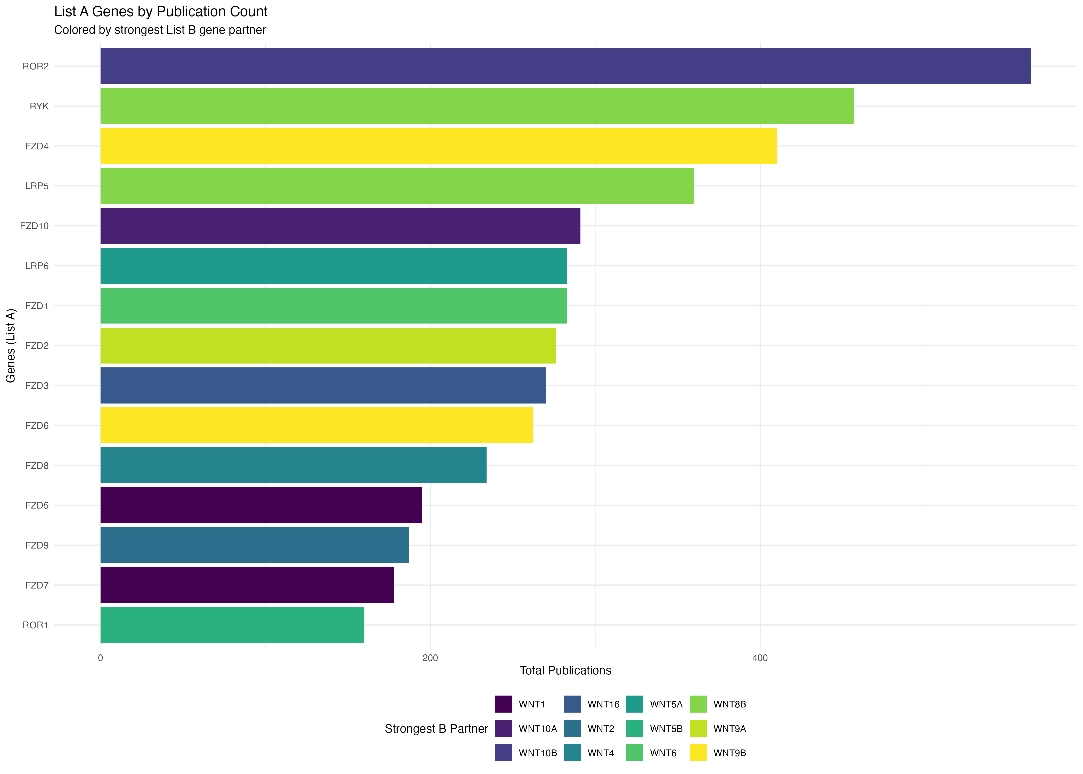

print(p2)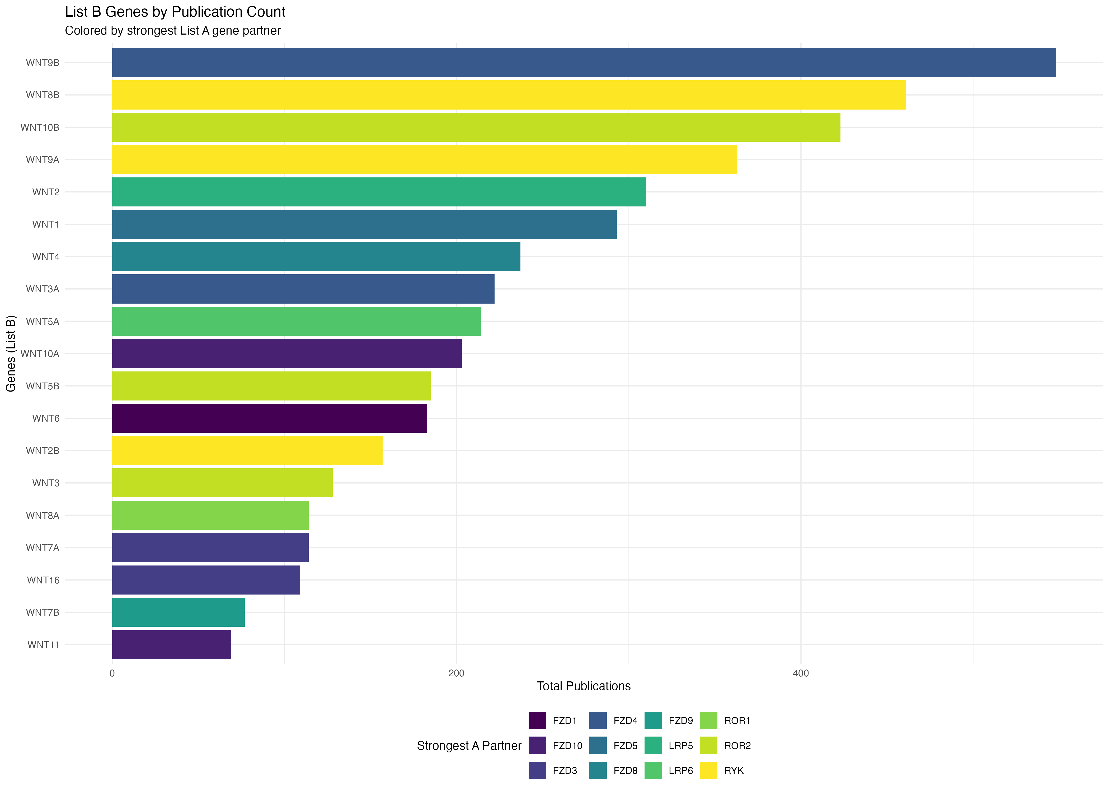

The full matrix

Raw PubMed publication counts for every ligand-receptor pair. Rows are FZD/LRP/ROR/RYK receptors, columns are WNT ligands.

kable(result,
  caption = "Co-occurrence Matrix: WNT Genes (Publication Counts)",
  align = "c",
  format = if (knitr::pandoc_to() == "html") "html" else "markdown"
) %>%
  kableExtra::kable_styling(
    bootstrap_options = c("striped", "hover", "condensed"),
    full_width = FALSE,
    position = "center"
  ) %>%
  kableExtra::add_header_above(c(" " = 1, "Wnt Genes" = length(A)))

Co-occurrence Matrix: WNT Genes (Publication Counts)
	Wnt Genes
	WNT1	WNT2	WNT2B	WNT3	WNT3A	WNT4	WNT5A	WNT5B	WNT6	WNT7A	WNT7B	WNT8A	WNT8B	WNT9A	WNT9B	WNT10A	WNT10B	WNT11	WNT16
FZD1	43	17	11	28	45	28	38	18	15	13	13	10	8	9	6	14	14	15	5
FZD2	15	24	11	12	30	26	89	22	8	11	15	6	6	5	2	5	13	15	4
FZD3	10	7	8	13	15	13	37	14	7	11	5	4	5	2	3	7	6	13	2
FZD4	12	26	14	17	33	18	44	14	11	19	20	9	6	5	3	5	11	16	4
FZD5	14	16	14	12	31	13	75	12	8	15	12	7	6	2	5	10	9	14	5
FZD6	11	14	12	17	22	21	49	14	6	12	12	6	5	3	3	8	13	22	4
FZD7	14	15	14	26	36	7	46	15	11	17	14	8	5	7	4	6	11	27	2
FZD8	10	7	6	12	21	6	20	8	7	3	6	14	5	4	3	6	9	9	0
FZD9	7	8	4	4	6	4	12	5	6	8	3	1	3	2	1	2	6	3	2
FZD10	9	5	10	11	16	10	17	8	12	8	15	9	7	3	2	10	9	11	6
LRP5	102	23	12	61	190	32	82	10	5	17	27	5	8	10	7	10	38	13	21
LRP6	87	21	13	56	237	30	76	13	8	24	21	13	10	6	13	26	38	21	8
ROR1	2	1	2	3	10	2	110	11	0	1	0	1	1	1	0	1	2	3	2
ROR2	14	6	2	13	35	7	327	16	2	8	1	7	2	2	0	4	3	17	2
RYK	9	4	1	9	12	9	64	10	0	2	0	2	1	1	0	1	1	8	0

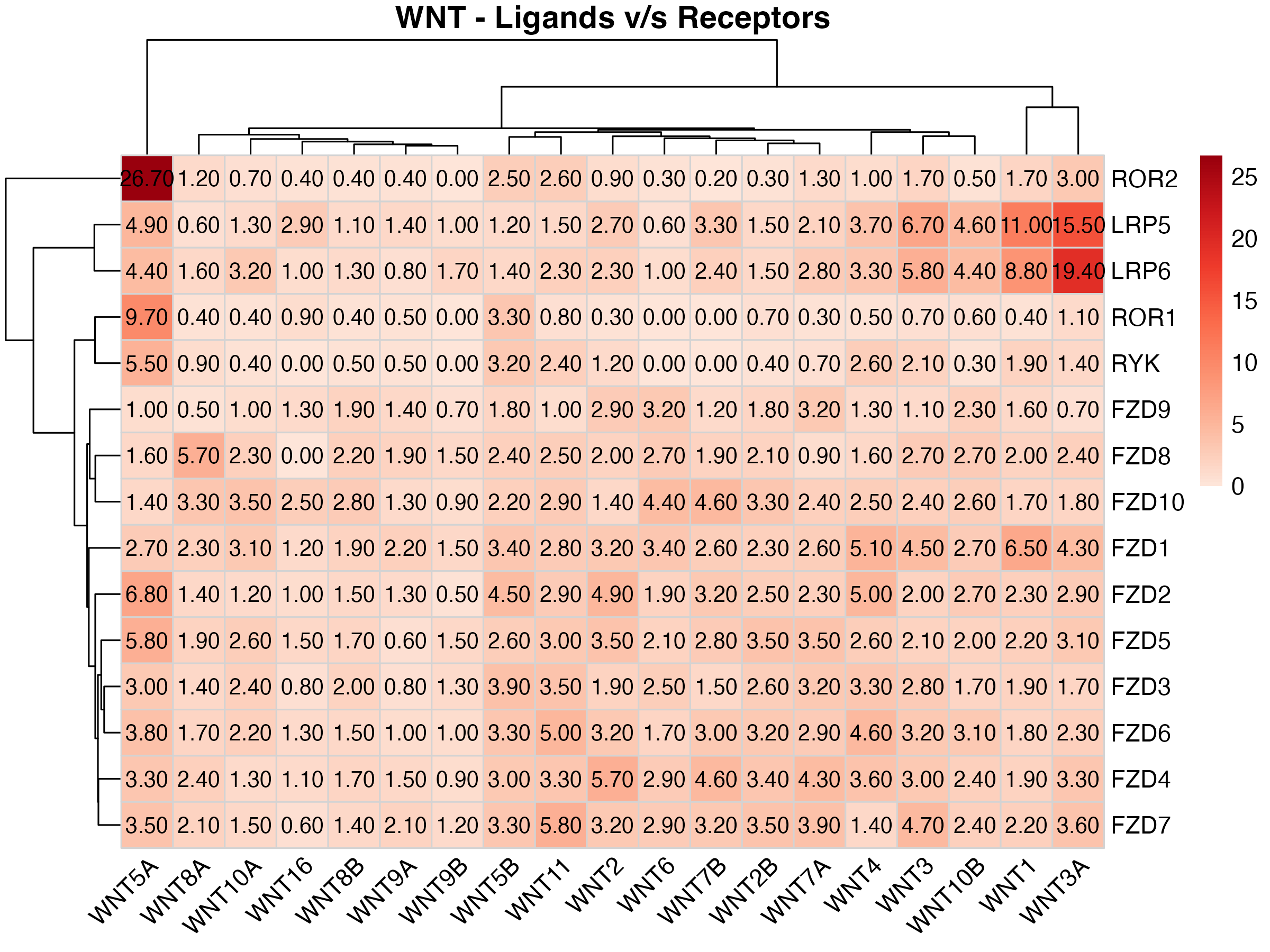
Heatmaps

A 15x19 table of numbers is hard to scan, so the heatmap below shows the same data with color instead. show_numbers = TRUE keeps the counts visible in each cell for reference.

plot_pubmatrix_heatmap(
  matrix = result,
  title = "WNT - Ligands v/s Receptors",
  show_numbers = TRUE
)

Dropping the numbers makes the overall pattern easier to read at a glance, which is useful when the shape of the relationship matters more than exact counts.

pubmatrix_heatmap(matrix = result)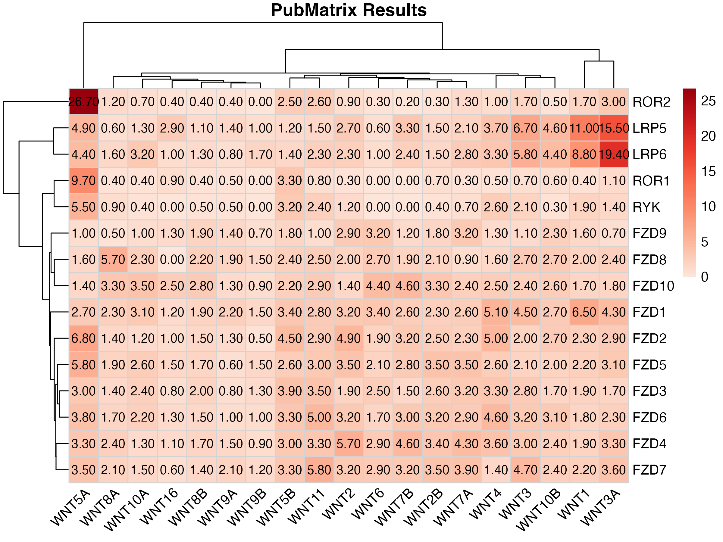

System Information

sessionInfo()

## R version 4.6.0 (2026-04-24)
## Platform: aarch64-apple-darwin23
## Running under: macOS Tahoe 26.5.1
## 
## Matrix products: default
## BLAS:   /Library/Frameworks/R.framework/Versions/4.6/Resources/lib/libRblas.0.dylib 
## LAPACK: /Library/Frameworks/R.framework/Versions/4.6/Resources/lib/libRlapack.dylib;  LAPACK version 3.12.1
## 
## locale:
## [1] C.UTF-8/C.UTF-8/C.UTF-8/C/C.UTF-8/C.UTF-8
## 
## time zone: Europe/London
## tzcode source: internal
## 
## attached base packages:
## [1] stats     graphics  grDevices utils     datasets  methods   base     
## 
## other attached packages:
## [1] ggplot2_4.0.3    pheatmap_1.0.13  dplyr_1.2.1      kableExtra_1.4.0
## [5] knitr_1.51       PubMatrixR_1.0.0
## 
## loaded via a namespace (and not attached):
##  [1] sass_0.4.10        generics_0.1.4     xml2_1.6.0         stringi_1.8.7     
##  [5] digest_0.6.39      magrittr_2.0.5     evaluate_1.0.5     grid_4.6.0        
##  [9] RColorBrewer_1.1-3 fastmap_1.2.0      jsonlite_2.0.0     viridisLite_0.4.3 
## [13] scales_1.4.0       pbapply_1.7-4      textshaping_1.0.5  jquerylib_0.1.4   
## [17] cli_3.6.6          rlang_1.2.0        withr_3.0.3        cachem_1.1.0      
## [21] yaml_2.3.12        otel_0.2.0         tools_4.6.0        parallel_4.6.0    
## [25] readODS_2.3.5      curl_7.1.0         vctrs_0.7.3        R6_2.6.1          
## [29] lifecycle_1.0.5    stringr_1.6.0      fs_2.1.0           htmlwidgets_1.6.4 
## [33] ragg_1.5.2         pkgconfig_2.0.3    desc_1.4.3         pkgdown_2.2.0     
## [37] bslib_0.11.0       pillar_1.11.1      gtable_0.3.6       glue_1.8.1        
## [41] systemfonts_1.3.2  xfun_0.59          tibble_3.3.1       tidyselect_1.2.1  
## [45] rstudioapi_0.19.0  farver_2.1.2       htmltools_0.5.9    labeling_0.4.3    
## [49] rmarkdown_2.31     svglite_2.2.2      compiler_4.6.0     S7_0.2.2

A comprehensive guide to analyzing publication relationships

ToledoEM